ParametricFunction class
object > Container > Mobject > VMobject > ParametricFunction
manimlib.mobject.functions.ParametricFunction(self, function=None, **kwargs)Create a Manim object using the given function. The function is an expression for the position value of the Manim coordinate system.
    CONFIG = {
        "t_min": 0,
        "t_max": 1,
        "step_size": 0.01,  # Use "auto" (lowercase) for automatic step size
        "dt": 1e-8,
        # TODO, be smarter about figuring these out?
        "discontinuities": [],
    }
Parameters: function=None
    Function used for object creation.
    The function is expressed by a formula indicating which point value in the screen
    corresponds to the variable t.

Parameters: **kwargs
    CONFIG values of ParametricFunction and VMobject/Mobject

    - t_min=0: Minimum input value

    - t_max=1: Maximum input value

    - step_size=0.01: Incremental value of input.
                      The function value is obtained by increasing the input value
                      according the this step size .
                      If step_size="auto", its value is automatically calculated
                      (if x is between -1 to 1 then 0.01, else log10(x))

    - stroke_color=None: Graph line color

    - stroke_width=DEFAULT_STROKE_WIDTH=4: Graph line thickness
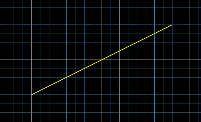
Let's draw a graph using a simple function.
The equation of function is $y=0.5x$
If you create a lambda function using this equation,
func1 = lambda t: np.array([t, 0.5 * t, 0])Manim's object is a group of points, and the points are represented by np.array, so if the x-axis value is t, the y value at this time becomes 0.5 * t, so np.array([t, 0.5 * t, 0 ]).
Let's make ParametricFucntion above func1 function.
        graph1 = ParametricFunction(
            func1,
            t_min=-4,
            t_max=4,
            color=YELLOW,
        )
When the x-axis value changes from -4 to 4, a graph is plotted with the YELLOW line of func1.

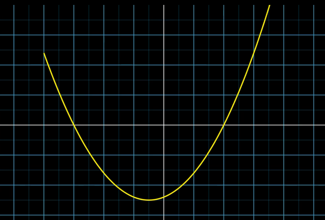
Let's create a quadratic function.
Let's create a quadratic function.
When x=-3 and x=2, it meets the x-axis and is a convex downward graph. In the formula, $y=0.4(x+3)(x−2)$
Multiplying by 0.4 is to prevent the y value from getting too large, so it is off the screen.
Let's create lambda function and ParametricFunction using the above formula.
        func2 = lambda t: np.array([t, 0.4*(t+3)*(t-2), 0])

        graph2 = ParametricFunction(
            func2,
            t_min=-4,
            t_max=4,
            color=YELLOW,
        )

The full source code is below.
class ParametricFunctionTest(Scene):
    def construct(self):

        self.add(NumberPlane())
        self.para_function1()

    def para_function1(self):
        func1 = lambda t: np.array([t, 0.5 * t,0])
        func2 = lambda t: np.array([t, 0.4*(t+3)*(t-2), 0])

        graph1 = ParametricFunction(
            func1,
            t_min=-4,
            t_max=4,
            color=YELLOW,
        )

        graph2 = ParametricFunction(
            func2,
            t_min=-4,
            t_max=4,
            color=YELLOW,
        )

        # self.add(graph1, graph2)
        self.add(graph2)
        self.wait()
I did self.add(NumberPlane()) in the source code to show a grid in the background. NumberPlane is covered in the following [05-5-D] Grid Background: NumberPlane page.
In the example above, we put a general mathematical expression into x, y of np.array, such as 'func1 = lambda t: np.array([t, 0.5 * t, 0])', so that the return value of the function is np.array type value.
You can also put it directly into the formula of a normal vector. The same expression as above,
func1 = lambda t: ( RIGHT + 0.5 * UP) * t
Geometrically, the meaning of this expression is multiplied by t for the vector of the point that moves one unit to the right and moves 0.5 unit upward. If you think about the graph shape of $y=0.5x$, it will make sense.
The code written in this way is as follows, and the output graph will be the same.
    def para_function2(self):
        func1 = lambda t: ( RIGHT + 0.5 * UP) * t
        graph1 = ParametricFunction(
            func1,
            t_min=-4,
            t_max=4,
            color=YELLOW,
        )

        self.add(graph1)
        self.wait()
It is more convenient to use because the method of expressing the general formula in x and y of np.array is intuitive. FunctionGraph is a class created to create graphs using these general mathematical formulas.
FunctionGraph class
object > Container > Mobject > VMobject > ParametricFunction > FunctionGraph
manimlib.mobject.functions.FunctionGraph(self, function, **kwargs)Create a Manim object using the given 'function'. The 'function' contains a general mathematical formula using x, y
    CONFIG = {
        "color": YELLOW,
        "x_min": -FRAME_X_RADIUS,
        "x_max": FRAME_X_RADIUS,
    }
Parameters: function
    Function used for object creation.
    Function expression indicating what y is for the variable x

Parameters: **kwargs
    CONFIG values of FunctionGraph and ParametricFunction/VMobject/Mobject

    - x_min=-FRAME_X_RADIUS: Minimum value of input

    - x_max=FRAME_X_RADIUS: Maxmimum value of input

    - color=YELLOW: Graph line color

    - step_size=0.01: Incremental value of input.
                      The function value is obtained by increasing the input value
                      according the this step size .
                      If step_size="auto", its value is automatically calculated
                      (if x is between -1 to 1 then 0.01, else log10(x))

    - stroke_width=DEFAULT_STROKE_WIDTH=4:  Graph line thickness
This is the most commonly used class for graph generation, because we can create graphs using function expressions by x and y familiar to us.
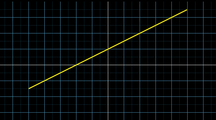
Let's draw a $y=ax+b$ function formula that can be called the simplest graph.

class FrunctionGraphTest(MovingCameraScene):
    def construct(self):
        self.add(NumberPlane())

    def simple_func(self):
        graph = FunctionGraph(
            lambda x: 0.5 * x + 1,
            x_min = -5,
            x_max = 5,
            color = YELLOW,
            stroke_width = 6,
        )
        self.play(ShowCreation(graph))
The function expression is a lambda expression, expressed as $lambda x: 0.5 * x + 1$, which represents $y=0.5x+1$
If you look at the graph, the slope is 0.5 and y-intercept is 1. It is well drawn according to the formula.
By adjusting the values of x_min and x_max, you can determine the range in which the graph is drawn, and with color you can change the graph line color, and with stroke_width you can change line thickness.
(Please change each value and get used to it.)
In the source code above, we used MovingCameraScene, but you can just use Scene.
Here, we only used MovingCameraScene for the purpose of enlarging the portion of the graph.
In addition, a grid line was drawn on the screen to know where the graph was located on the screen. This is done by NumberPlane(). There is no problem in creating a graph even if you remove it.
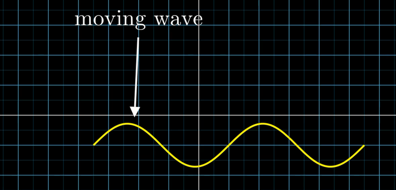
Let's do an example of creating a sine graph and changing the size and position of the graph.
    def sine_curve(self):
        curve = FunctionGraph(
            lambda t: np.sin(t),
            x_min=-TAU,
            x_max=TAU,
            color=YELLOW,
            stroke_width=6,
        )
        curve.move_to(DR)
        curve.set_width(9)

        equation = TextMobject("moving wave")
        equation.scale(1.5)
        equation.to_edge(UP)
        equation.shift(2 * LEFT)
        arrow = Arrow(
            equation.get_bottom(),
            curve.point_from_proportion(0.15)
        )

        self.play(
            ShowCreation(curve),
            Write(equation, run_time=1),
            GrowArrow(arrow),
        )
        self.wait()
The sine function is expressed as $lambda t: np-sin(t)$, and the range of x is from -2PI to 2PI. (TAU=2PI)
The graph created by FunctionGraph would be a typical sine graph going through the origin, which was moved to the lower right corner UR=[1,1] and forced the length to become 9.
        curve.move_to(DR)
        curve.set_width(9)

All of the graphs shown above are drawn in the range of x between [-7.1, 7.1] and the vertical range of y between [-4,4]. What if you want to make the x or y range bigger?
You cannot change the screen's coordinate system itself.
Instead, you can create a new axis with a virtual coordinate system to expand the range, draw a graph on the actual screen, with the scale ratio of the coordinates on this to the actural screen coordinates.
It's a little complicated in words, but if you look at the next chapter [05-5-B] Graph Line: NumberLine and [05-5-C] Graph Coordinate: Axes will make sense.
Next: [05-5-B] Graph Line: NumberLine
[05-5-B] Graph Line: NumberLine
In this page, we will look at the NumberLine responsible for the axis line, such as the x-axis and y-axis of the graph. The axis is not only responsible for drawing the horizontal line corresponding..
infograph.tistory.com
Go To: [99] Table of Contents
'Programming > Manim Lectures' 카테고리의 다른 글
| [05-5-C] Graph Coordinate: Axes (0) | 2020.06.07 |
|---|---|
| [05-5-B] Graph Line: NumberLine (0) | 2020.06.07 |
| [05-5] Graph (0) | 2020.06.07 |
| [05-4-B] Integer (0) | 2020.06.07 |
| [05-4-A] DecimalNumber (0) | 2020.06.07 |


